“Racorn-k”版本间的差异
(→Experiments on several datasets) |
(→Experiments on several datasets) |
||
| 第58行: | 第58行: | ||
=Experiments on several datasets= | =Experiments on several datasets= | ||
| − | + | ------------------------------------------------------------------------------------------------------------------ | |
| − | + | | Dataset DJIA MSCI SP500(N) HSI SP500(O) | |
| − | + | ------------------------------------------------------------------------------------------------------------------ | |
| − | + | | Criteria RET SR MDD | RET SR MDD | RET SR MDD | RET SR MDD | RET SR MDD | |
| − | + | Main |RACORN(C)-K 0.93 0.01 0.32 | 78.38 3.73 0.21 | 12.55 0.77 0.53 | 202.04 1.60 0.28 | 7.13 1.28 0.34 | |
| − | + | Results | RACORN-K 0.83 -0.19 0.37 | 79.52 3.67 0.21 | 13.03 0.72 0.57 | 264.02 1.60 0.29 | 9.27 1.33 0.32 | |
| − | + | | CORN-K 0.80 -0.24 0.38 | 77.54 3.63 0.21 | 12.50 0.70 0.60 | 254.27 1.56 0.30 | 8.72 1.26 0.35 | |
| − | + | ------------------------------------------------------------------------------------------------------------------ | |
| − | Naive | + | Naive | UBAH 0.76 -0.43 0.39 | 0.90 0.02 0.65 | 1.52 0.24 0.50 | 3.54 0.53 0.58 | 1.33 0.36 0.46 |
| − | + | Methods | UCRP 0.81 -0.28 0.38 | 0.92 0.05 0.64 | 1.78 0.28 0.68 | 4.25 0.58 0.55 | 1.64 0.55 0.31 | |
| − | + | ------------------------------------------------------------------------------------------------------------------ | |
| − | Follow the | + | Follow the | UP 0.81 -0.29 0.38 | 0.92 0.04 0.64 | 1.79 0.29 0.68 | 4.26 0.59 0.55 | 1.66 0.56 0.31 |
| − | Winner | + | Winner | EG 0.81 -0.29 0.38 | 0.92 0.04 0.64 | 1.75 0.28 0.67 | 4.22 0.58 0.55 | 1.62 0.54 0.32 |
| − | + | | ONS 1.53 0.80 0.32 | 0.85 0.02 0.68 | 0.78 0.27 0.96 | 4.42 0.52 0.68 | 3.32 1.11 0.25 | |
| − | + | ------------------------------------------------------------------------------------------------------------------ | |
| − | + | | ANTICOR 1.62 0.85 0.34 | 2.75 0.96 0.51 | 1.16 0.24 0.93 | 9.10 0.74 0.56 | 5.58 1.08 0.38 | |
| − | + | | ANTICOR2 2.28 1.24 0.35 | 3.20 1.02 0.48 | 0.71 0.22 0.97 | 12.27 0.77 0.55 | 5.86 1.01 0.49 | |
| − | Follow the | + | Follow the | PAMR2 0.70 -0.15 0.76 | 16.73 2.07 0.54 | 0.01 -0.28 1.00 | 1.19 0.20 0.86 | 4.97 0.90 0.51 |
| − | Loser | + | Loser | CWMR Stdev 0.69 -0.17 0.76 | 17.14 2.07 0.54 | 0.02 -0.26 0.99 | 1.28 0.22 0.85 | 5.92 0.96 0.51 |
| − | + | | OLMAR1 2.53 1.16 0.37 | 14.82 1.85 0.48 | 0.03 -0.11 1.00 | 4.19 0.46 0.77 | 15.89 1.28 0.41 | |
| − | + | | OLMAR2 1.16 0.40 0.58 | 22.34 2.08 0.42 | 0.03 -0.11 1.00 | 3.65 0.43 0.84 | 9.54 1.08 0.49 | |
| − | + | ------------------------------------------------------------------------------------------------------------------ | |
| − | Pattern | + | Pattern | BK 0.69 -0.68 0.43 | 2.62 1.06 0.51 | 1.97 0.31 0.59 | 13.90 0.88 0.45 | 2.21 0.64 0.49 |
| − | Matching | + | Matching | BNN 0.88 -0.15 0.31 | 13.40 2.33 0.33 | 6.81 0.67 0.41 | 104.97 1.40 0.33 | |
| − | + | ------------------------------------------------------------------------------------------------------------------ | |
=View the impact of risk-aversion= | =View the impact of risk-aversion= | ||
2017年10月31日 (二) 02:48的版本
目录
Project name
RACORN-K: RISK-AVERSION PATTERN MATCHING-BASED PORTFOLIO SELECTION
Project members
Yang Wang, Dong Wang, Yaodong Wang, You Zhang
Introduction
Portfolio selection is the central task for assets management, but it turns out to be very challenging. Methods based on pattern matching, particularly the CORN-K algorithm, have achieved promising performance on several stock markets. A key shortage of the existing pattern matching methods, however, is that the risk is largely ignored when optimizing portfolios, which may lead to unreliable profits, particularly in volatile markets. To make up this shortcoming, We propose a risk-aversion CORN-K algorithm, RACORN-K, that penalizes risk when searching for optimal portfolios. Experiment results demonstrate that the new algorithm can deliver notable and reliable improvements in terms of return, Sharp ratio and maximum drawdown, especially on volatile markets.
Corn-k
At the t-th trading period, the CORN-K algorithm first selects all the historical periods whose market status is similar to that of the present market, where the similarity is measured by the Pearson correlation coefficient. This patten matching process produces a set of similar periods, which we denote by C. Then do a optimization following the idea of BCRP[] on C. Finally, the outputs of the top-k experts that have achieved the highest accumulated return are weighted to derive the ensemble-based portfolio.
Racorn-k
At the t-th trading period, the CORN-K algorithm first selects all the historical periods whose market status is similar to that of the present market, where the similarity is measured by the Pearson correlation coefficient. This patten matching process produces a set of similar periods, which we denote by C. Then do a optimization following the idea of BCRP[] on C. Finally, the outputs of the top-k experts that have achieved the highest accumulated return are weighted to derive the ensemble-based portfolio.
Racorn(c)-k
At the t-th trading period, the CORN-K algorithm first selects all the historical periods whose market status is similar to that of the present market, where the similarity is measured by the Pearson correlation coefficient. This patten matching process produces a set of similar periods, which we denote by C. Then do a optimization following the idea of BCRP[] on C. Finally, the outputs of the top-k experts that have achieved the highest accumulated return are weighted to derive the ensemble-based portfolio.
Experiments on several datasets
------------------------------------------------------------------------------------------------------------------
           |  Dataset          DJIA              MSCI             SP500(N)             HSI             SP500(O)
------------------------------------------------------------------------------------------------------------------
           | Criteria     RET   SR   MDD |  RET   SR   MDD |  RET    SR   MDD |  RET    SR   MDD |  RET   SR   MDD
Main       |RACORN(C)-K  0.93  0.01 0.32 | 78.38 3.73 0.21 | 12.55  0.77 0.53 | 202.04 1.60 0.28 |  7.13 1.28 0.34
Results    |  RACORN-K   0.83 -0.19 0.37 | 79.52 3.67 0.21 | 13.03  0.72 0.57 | 264.02 1.60 0.29 |  9.27 1.33 0.32
           |   CORN-K    0.80 -0.24 0.38 | 77.54 3.63 0.21 | 12.50  0.70 0.60 | 254.27 1.56 0.30 |  8.72 1.26 0.35
------------------------------------------------------------------------------------------------------------------
Naive      |    UBAH     0.76 -0.43 0.39 |  0.90 0.02 0.65 |  1.52  0.24 0.50 |   3.54 0.53 0.58 |  1.33 0.36 0.46
Methods    |    UCRP     0.81 -0.28 0.38 |  0.92 0.05 0.64 |  1.78  0.28 0.68 |   4.25 0.58 0.55 |  1.64 0.55 0.31
------------------------------------------------------------------------------------------------------------------
Follow the |     UP      0.81 -0.29 0.38 |  0.92 0.04 0.64 |  1.79  0.29 0.68 |   4.26 0.59 0.55 |  1.66 0.56 0.31
Winner     |     EG      0.81 -0.29 0.38 |  0.92 0.04 0.64 |  1.75  0.28 0.67 |   4.22 0.58 0.55 |  1.62 0.54 0.32
           |     ONS     1.53  0.80 0.32 |  0.85 0.02 0.68 |  0.78  0.27 0.96 |   4.42 0.52 0.68 |  3.32 1.11 0.25
------------------------------------------------------------------------------------------------------------------
           |  ANTICOR    1.62  0.85 0.34 |  2.75 0.96 0.51 |  1.16  0.24 0.93 |   9.10 0.74 0.56 |  5.58 1.08 0.38
           |  ANTICOR2   2.28  1.24 0.35 |  3.20 1.02 0.48 |  0.71  0.22 0.97 |  12.27 0.77 0.55 |  5.86 1.01 0.49
Follow the |   PAMR2     0.70 -0.15 0.76 | 16.73 2.07 0.54 |  0.01 -0.28 1.00 |   1.19 0.20 0.86 |  4.97 0.90 0.51
Loser      | CWMR Stdev  0.69 -0.17 0.76 | 17.14 2.07 0.54 |  0.02 -0.26 0.99 |   1.28 0.22 0.85 |  5.92 0.96 0.51
           |   OLMAR1    2.53  1.16 0.37 | 14.82 1.85 0.48 |  0.03 -0.11 1.00 |   4.19 0.46 0.77 | 15.89 1.28 0.41
           |   OLMAR2    1.16  0.40 0.58 | 22.34 2.08 0.42 |  0.03 -0.11 1.00 |   3.65 0.43 0.84 |  9.54 1.08 0.49
------------------------------------------------------------------------------------------------------------------
Pattern    |     BK      0.69 -0.68 0.43 |  2.62 1.06 0.51 |  1.97  0.31 0.59 |  13.90 0.88 0.45 |  2.21 0.64 0.49
Matching   |     BNN     0.88 -0.15 0.31 | 13.40 2.33 0.33 |  6.81  0.67 0.41 | 104.97 1.40 0.33 |
------------------------------------------------------------------------------------------------------------------
View the impact of risk-aversion
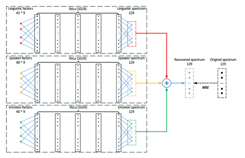
To verify the factorization, we can reconstruct the speech signal from the factors. The reconstruction is simply based on a DNN, as shown below. Each factor passes a unique deep neural net, the output of the three DNNs are added together, and compared with the target, which is the logarithm of the spectrum of the original signal. This means that the output of the DNNs of the three factors are assumed to be convolved together to produce the original speech.
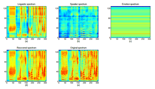
Note that the factors are learned from Fbanks, by which some speech information has been lost, however the recovery is rather successfull.
View the reconstruction
Reference
[1] Lantian Li, Yixiang Chen, Ying Shi, Zhiyuan Tang, and Dong Wang, “Deep speaker feature learning for text-independent speaker verification,”, Interspeech 2017.
[2] Ehsan Variani, Xin Lei, Erik McDermott, Ignacio Lopez Moreno, and Javier Gonzalez-Dominguez, “Deep neural networks for small footprint text-dependent speaker verification,”, ICASSP 2014.
[3] Lantian Li, Dong Wang, Yixiang Chen, Ying Shing, Zhiyuan Tang, http://wangd.cslt.org/public/pdf/spkfact.pdf
[4] Lantian Li, Zhiyuan Tang, Dong Wang, FULL-INFO TRAINING FOR DEEP SPEAKER FEATURE LEARNING, http://wangd.cslt.org/public/pdf/mlspk.pdf
[5] Zhiyuan Thang, Lantian Li, Dong Wang, Ravi Vipperla "Collaborative Joint Training with Multi-task Recurrent Model for Speech and Speaker Recognition", IEEE Trans. on Audio, Speech and Language Processing, vol. 25, no.3, March 2017.
[6] Dong Wang,Lantian Li,Ying Shi,Yixiang Chen,Zhiyuan Tang., "Deep Factorization for Speech Signal", https://arxiv.org/abs/1706.01777

